Showing posts with label Research. Show all posts

Friday, April 9, 2010

Research (Nuts and Bolts)

I have been trying to work with hadoop for my parallelization needs, but I find it to be somewhat difficult to get certain things to work in the system. At University of Rochester, CS, the cluster that I work with doesn't seem to have OpenMPI or any kind of MPI set up on the cluster machines, but at Montreal, the machines do, except that all of the nodes (except for usually 5) are always used by some crystallography program that seems to eats bandwidth and I/O on the NFS filesystem. So I've been doing stuff and copying back and forth, which was just killing me. (Not because it was taking so long and being difficult to do, but the principle damnit!)

So I was avoiding installing openmpi on the Rochester system because I figured it would be difficult at best, and impossible at worst. But eventually I gave up on getting hadoop to play nice and find that it is remarkably easy to set up OpenMPI on a given cluster. If you have a cluster with a common NFS mount, all you have to do is download and unpack and set your path to wherever you installed openmpi. Let me just blog this in case you're wondering how to go about it.

First, I downloaded the tarball from here and unpacked it into ~/openmpi. Then in that directory,

$./configure --prefix=/u/rim/opt/openmpi
$ make all install

Thats pretty much it, other than setting

PATH=$PATH:/u/rim/opt/openmpi/bin
LD_LIBRARY_PATH=$LD_LIBRARY_PATH:/u/rim/opt/openmpi/lib

in my .bashrc file. YMMV depending on your favorite shell.

Now I had to write my MPI program, which actually I already did, but here it is for completeness, or at least the main function. This generates a kernel matrix, which is relatively easy to do parallel, I just give row indices of the test matrix to each node and ask them politely to kernelize that part of the final matrix.

When they're done they send them back to the master node, which copies these columns into the big matrix. The only tricky part with ublas is to make sure that the MPI receive and send copy the respective right parts of the matrix. Here, since we're copying rows of the final kernel matrix, we want everything to be row major.

int main(int argc, char *argv[]){
 
  matrix<double> Xtrain;
  matrix<double> Ytrain;
  matrix<double> Xtest;
  matrix<double> Ytest;

  MPI_Status status;
  int size = 1;
  int rank = 0;

  MPI_Init(&argc, &argv);
  size = MPI::COMM_WORLD.Get_size();
  rank = MPI::COMM_WORLD.Get_rank();

  char name[MPI_MAX_PROCESSOR_NAME];
  int len;
  memset(name,0,MPI_MAX_PROCESSOR_NAME);
  MPI::Get_processor_name(name,len);
  memset(name+len,0,MPI_MAX_PROCESSOR_NAME-len);

  if(!load_data(argv[1], Xtrain, Ytrain)){
    cout << "klr_test (error): Bad train filename" << endl;
    return 0;
  }

  if(!load_data(argv[2], Xtest, Ytest)){
    cout << "klr_test (error): Bad test filename" << endl;
    return 0;
  }

  kernelType kernel = RBF;
  if(string(argv[3]) == "CHI2"){
    kernel = CHI2;
  }
  if(string(argv[3]) == "POLY"){
    kernel = POLY;
  }
  if(string(argv[3]) == "LINEAR"){
    kernel = LINEAR;
  }
  if(string(argv[3]) == "EUCLIDEAN"){
    kernel = EUCLIDEAN;
  }

  double param1 = atof(argv[4]);
  int N = Xtest.size1();
  int D = Xtrain.size1();

  //split the matrix into row matrices
  int offset = floor((double)N / (double)size);
  int start = rank*offset;
  int end = (rank+1)*offset;
  end = end > N ? N : end;
  int M = end - start;
  if(rank + 1 == size){
    end = N;
    M = end - start;
  }


  ublas::matrix<double, ublas::row_major> K(N, D);

  if(rank == 0){
    K.assign(ublas::zero_matrix<DBL_TYPE>(N, D));
  }else{
    K.resize(M, D, false);
    K.assign(ublas::zero_matrix<DBL_TYPE>(M, D));
  }


  for(int k = start; k < end; k++){
    matrix_row< matrix<double> > u1(Xtest, k);
    int j = k - start;
    for(int i = 0; i < D; i++){
      matrix_row< matrix<double> > u2(Xtrain, i);
      K(j, i) = kernelize(u1, u2, kernel, param1);
    }
    if(VERBOSE && (k % 100 == 0))
      std::cout << k << ": " << rank << " " << name << std::endl;
  }

 if(size > 1){
    if(rank == 0){
      for(int i = 1; i < size; i++){
        start = i*offset;
        end = (i+1)*offset;
        end = end > N ? N : end;
        M = end - start;
        if(i+1 == size){
          end = N;
          M = end - start;
        }
        MPI_Recv((void *)&K.data()[start*D], M*D, MPI_DOUBLE, i, TAG_MATRIX_PARTITION, MPI_COMM_WORLD, &status);
      }
    }else{
      MPI_Send((void *)&K.data()[0], M*D, MPI_DOUBLE, 0, TAG_MATRIX_PARTITION, MPI_COMM_WORLD);
    }
  }


  if(rank == 0){
    ofstream output(argv[5], ios::out);
    for(unsigned int i = 0; i < K.size1(); i++){
      for(unsigned int j = 0; j < K.size2(); j++){
        output << K(i, j);
        if(j < (K.size2()-1)){
          output << ",";
        }
      }
      output << std::endl;
    }
  }

  MPI_Finalize();
  return 0;
}

Now to make and run, just edit your Makefile to do something like

MPICC=mpic++
...
$(MPICC) kernelize_mat2.cpp -o kernelize_mat2 $(LFLAGS) $(CFLAGS) $(INC) $(OLIBS)

where everything to the right of -o kernelize_mat2 are just settings and flags I otherwise needed. The only change I made was to add the mpi wrapper for the g++ compiler, mpic++. The other bits are stuff that I already had/needed.

After building, you can run. On the cluster, they use Torque for scheduling, so you can either do it via shell script or via the interactive start. I generally prefer to use the shell script since it's less wasteful, but here I use the interactive start up because I wanted to make sure it was all kosher.

$ qsub -I -lnodes=5,walltime=3600,mem=1000M

I like to use funny names for my pbs jobs, but I skip that here. That command line requests 5 nodes with an hour of cpu time and a gig of memory each, which is about what I wanted.

$ mpirun -np 5 --hostfile $PBS_NODEFILE /path/to/kernelize_mat2 train.csv test.csv RBF .7 kernel.csv

-np tells how many processors you want to use and the --hostfile $PBS_NODEFILE says which hosts you want to run your process on. You can, of course use less, but thats a little silly, no? You can also run it locally if you exclude hosts in the hostfile. That is you can also specify

-np 4 --host node33
In any case at each step I was expecting the thing to say, root access required or something, but I guess that's being silly. Anyways, the whole thing worked like a charm and took roughly 20 minutes to set up and get running (almost all of that time was spent compiling).

That's pretty much it, so now you too can write cool apps for the cluster, and if you're using the one I use, then by all means, you can just set your paths to mine (although names were changed to protect the innocent). By the way, does this code really need comments? I don't even know where I would put one.

Wednesday, March 3, 2010

Research (converting to cblas, a note to future me)

So while I wait for a bunch of tests to complete, I figured I would write this on here for future me.

Hi, Dave, if you're reading this, then you totally forgot how to do this. Lemme help you out.

Switching from boost::ublas to the blas/cblas interface made things much much faster. So here are what I did to convert boost::ublas implemented code to cblas in less than a few hours. There may be easier/better ways, but this worked for me and provided a nice gentle way for me to learn how to use the blas functions. Keep in mind that I don't have root access to these machines, so this works even if you only have access as a user.

First, I installed the cblas interface. I'm assuming you have liblapack installed somewhere or its equivalent, as well as gfortran.

Then unpack, and move into the CBLAS directory. Copy Makefile.<ARCH> into Makefile.in. Here I used Makefile.LINUX. The only sections I changed here was to

BLLIB = $(ACML_LINK) -L/opt/pgi/linux86-64/6.2/libso -lacml -lacml_mv -lpgftnrtl
CBDIR = $(HOME)/CBLAS
CBLIBDIR = $(CBDIR)/lib/$(PLAT)
CBLIB = $(CBLIBDIR)/cblas_$(PLAT).a
...
FC = gfortran

To add AMD's math libraries acml, acml_mv and pgftnrtl, a fortran runtime library, which are stored in that directory. Also, I didn't have g77 installed, so I used its updated version, gfortran.

After this, just run

 
$ make alllib
And you should get a nice static link library out called cblas_LINUX.a. This stores all the various blas level 1/2/3 interface objects in one container. You can make your executables smaller if you use individual objects.

Now, I just had to add

extern "C"{
#include "cblas.h"
}
To my header files, and I can now use the cblas functions.

To make my life easier, I ended up writing a bunch of wrappers for the cblas functions, here is an example.

void cblas_prod
 (ublas::matrix<double, ublas::row_major, ublas::unbounded_array<double> >& C,
  const ublas::matrix<double, ublas::row_major, ublas::unbounded_array<double> >& A,
  const ublas::matrix<double, ublas::row_major, ublas::unbounded_array<double> >& B){
  cblas_dgemm(CblasRowMajor,
              CblasNoTrans,
              CblasNoTrans,
              C.size1(), C.size2(), A.size2(),
              1.0,
              &A.data()[0],
              A.size2(),
              &B.data()[0],
              B.size2(),
              1.0,
              &C.data()[0],
              C.size2());
}
As you can see, the way the inner data array is arranged makes all the difference. In general, ublas's matrix and vector array can be accessed by its .data() member function. Since this is row major, each matrix row contains column size entries, so use the column size (A.size2()) as an argument to the int incX arguments in the cblas API. Alternatively if A were column major, you'd use A.size1() as the "incA" argument.

By adding one of these for every combination (rowMajor, rowMajor, colMajor), (rowMajor, colMajor, rowMajor), you can avoid the headache of caring when you just want to multiply two matrices. On the other hand, you should be aware that dgemm, for example can do a bit more than straight multiplication. Actually, also zero out the C matrix above before using, as written, the above actually assigns C = A*B + C, unless this is the behavior you want.

Now linking is pretty easy, and getting the right includes is pretty easy. Just set your makefile to do something like

$ g++ /path/to/cblas_LINUX.a myfile.cpp -o myfile.exe \
  -L. -L/opt/pgi/linux86-64/6.2/libso -lacml -lacml_mv -lpgftnrtl \ 
  -O3 -fexpensive-optimizations -funroll-loops -DNDEBUG \
  -I/where/you/unpacked/CBLAS/src -I. 
And now you can replace any slow ublas things with fast cblas things, without too much change.

Sincerely, me.

Sunday, February 28, 2010

Research

Ok, I'm an idiot. Just converted code to use CBlas instead of Ublas matrix multiplication, its ridiculously faster. Word to the wise. Forget about about boost::ublas, except maybe for storage.

Tuesday, February 23, 2010

Research

So, ok, I've put every trick I know into the mix and all my code seems like it's as optimized as possible, but I still have issues. The main problem is one matrix multiplication operation that I only have to once (not per iteration), but it is very expensive. Before I get rid of it completely, I'd really like to know how well it would work if I parallelized it.

However, doing this wasn't as easy as it seems. I have access to a 64-node cluster of quad-Xeons with 5 gigs each (I think, who knows). My matrix multiplication is $\mathbf{X}^T\mathbf{X}$, where $\mathbf{X}$ is a 810,000 by 275 double precision matrix assumed to be of full-rank.

I could conceivably do this on a single machine (quad CPU), but it seems pretty ripe to just parcel out rows of the matrix, compute the outer products on each node and then add each of these matrices up. The main issue is memory and IO, rather than the computation, so this seems better to do distributed than on multi-cpu.

Of course nothing is easy with limited resources. The cluster I'm working on doesn't seem to have MPI or MapReduce frameworks available. It uses Torque to manage jobs, which means I had to read a lot of man pages, write a bunch of shell scripts, and use the NFS mount for communication. So here's hoping if you're reading this, you can skip all that.

(I hate Perl, but in retrospect, I probably should've done this in Perl. I don't even hate Perl, I just hate Perl programmers. They tend to write code, well, cryptically, and seem proud of it. I hate the game, not the player. Jeff is nice.)

Anyways, I did shell. Since I didn't find good versions of this online, I'm putting this out there for all to make fun of.

First, I had two C-programs, which do the obvious computations

$ xtx_map file output
$ xtx_reduce dir output
xtx_map takes a matrix X, stored in file, and outputs X'X to output, and xtx_reduce takes a directory and computes a sum of all matrices stored as files there.

Now I had to get the data ready and set up for the matrices I needed. So I needed 3 shell scripts for this, a basic wrapper for all the calls, and a map shell script to call xtx_map and a reduce script to call xtx_reduce. Here's the wrapper.

#!/bin/sh
split=`which split`;
$split -l 10000 $SPLIT /u/dave/input/X_
scoreboard=/u/dave/scoreboard
for f in `ls /u/dave/input/X_*`; do
    used=`cat $scoreboard`
    export f=`basename $f`
    while [ $used -gt 30 ]; do
        used=`cat $scoreboard`
        echo "waiting for node to open up..."
        sleep 1
    done
    qsub -v FILENAME=$f /u/dave/scripts/map.sh
    used=`expr $used + 1`
    echo $used > $scoreboard
done
jobs=""
for job in `qstat -u dave | awk {'print $1'} | sed 's/\.node.*//' | grep '[0-9]'`; do
    nan="$(echo $job | sed 's/[0-9]//g')"
    if [ -z $nan ] ; then
        if [ -z $jobs ]; then
            export jobs=$job
        else
            export jobs=$jobs:$job
        fi
    fi
done
qsub -W depend=afterok:$jobs /u/dave/scripts/reduce.sh

So lines 2 & 3 call the unix tool split on the file I want to break up using 10000 lines per each submatrix and saving to the directory /u/dave/input/X_, in files name X_aa, X_ab, etc. (If you don't use split, it's awesome, and also you probably never used a 9600 baud modem. GTS.) "which" is also a nifty utility to use when people put common tools in weird places. Yeah, you heard me MacOSX.

Now one issue is that with .8M lines there are roughly 80 files output, and I'm really only allowed to use 32 of these nodes. So I had to create a way to schedule the jobs to go into the cluster. So I just used the hacky tmp file way to do it, and this actually did not work so well. There was some non-deterministic accounting...

Probably a recursive call would work better here, but shell recursion does not seem safe. In any case, no harm no foul, line 4 sets the tmp file, called scoreboard, and then we get all the split files in an outer loop.

Inside the for loop, I read the scoreboard and wait until I have less than 31. I kept it at a round number because I'm really lazy. Ok, so then it submits the job to the PBS manager, which schedules the job using qsub. Now qsub doesn't handle arguments, but it does handle environment variables, so this hacky

-v FILENAME=$f
is the only way I found to do this.

Now the reduce step has to wait for all the jobs to finish, so the idea here is to get a list of job ids, and pass them to qsub reduce.sh to get it to wait until all the jobs are out. I could also have polled or something, which would be safer, but this seemed OK to me, especially since I could have had the reduce step running concurrently, but this step is significanlty faster than the map steps, as we only need to add matrices of 275 by 275.

Finally after see-sawing between google and shell scripting, I got the right switches and stuff for the job to wait, which is

qsub -W depend=afterok:$jobs /u/dave/scripts/reduce.sh

The reduce and map shell scripts are pretty mundane: Map here:
#!/bin/sh
scoreboard=/u/dave/scoreboard
infile=/u/dave/input/$FILENAME
outfile=/u/dave/output/$FILENAME
/u/dave/bin/xtx_map $infile $outfile
used=`cat $scoreboard`
used=`expr $used - 1`
echo $used > $scoreboard
Reduce there:
#!/bin/sh
#PBS -m bea
indir=/u/dave/output
/u/dave/bin/xtx_reduce $indir /u/dave/XTX

I use the names map and reduce because it makes parallelization easy to think about, and I really hope I get some infrastructure that I can use Mapreduce with soon, because shell scripting sucks. Perhaps I'm very bad at it, but I just find it annoying and hacky.

Well, the good thing is that this code should work as a basis for any general problems. Hope this finds someone who it can help.

Saturday, February 6, 2010

Research

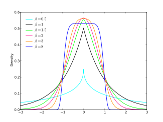
Wow, you'd think I wasn't getting any research done, but actually that's not quite the truth. I've packaged up a lot of things, tying up some loose ends. Here I'm going to describe a little about some work I've done with a distribution that I like I lot, called the Generalized Normal distribution, or Generalized Gaussian distribution.

Basically, the idea is that  $p(x) \propto \exp(-(\gamma(|x - \mu|)^\beta)$, so that with $\gamma = \frac{1}{2}\sigma^{-2}$, and $\beta = 2$, this is the Gaussian, and with $\beta=1$, we have a Laplace, or Exponential, depending on $\mu$.

The mean here is $\mu$ which is very nice, but the efficiency of the mean estimator (the average)  is quite different with different power. An intuitive understanding of what the generalization entails (what $\beta$ "means") is that the tail behavior changes. As $\beta$ approaches 0, we get heavier and heavier tails, and so intuitively, it becomes "harder" to estimate the mean. In fact, with $\mu = 0$, $\gamma = 1$, with $\beta$ less than about $1.4$, asymptotic variance of the median estimator is less than that of the mean estimator.

Weakening the assumption of exponential decay in the tails gives us a knob to twiddle in applications where we have might have a Gaussian prior, which is the most common prior for linear models. As is well known with the Exponential ($L_1$ regularization) prior, which are heavily peaked, if we assume mean 0, we can get sparse models. Moreover, we can show formally that effect of noise in the data will be limited, especially if we are interested in estimating median effects.

However, the Generalized Gaussian gives a nice way of managing the "peakiness" of the prior distribution, by allowing for different $\beta$ parameters to model the trade off between what we believe about how sparse the model is before seeing any data, and how much sparsity we actually desire.

This is just a short note about the prior, which I believe gives a nice way to go about parameterizing a prior for a linear model when what we care about is the smallest possible model, which is what we usually want.

This was just a short note about my favorite distributions.


Monday, January 18, 2010

Research

The $L_2$ regularized log conditional likelihood for kernel logistic regression is given as $\mathcal{L}(\mathbf{w}) = \sum_i \log(\sigma(y_i\mathbf{K}_i^T\mathbf{w})) - \frac{\lambda}{2}\mathbf{w}^T\mathbf{K}\mathbf{w}$ where $\mathbf{K}$is a Gramm matrix composed of the products $\mathbf{K}(i,j) = \langle \phi(\mathbf{x}_i), \phi(\mathbf{x}_j) \rangle$, $\lambda$represents a weight on the regularization penalty, and $\sigma(a) = (1 + \exp(-a))^{-1}$is the sigmoid logistic function.

The IVM [1] iteratively increase the number of basis functions $K_i$ used in the kernel expansion until $\mathcal{L}$converges. Letting $k$index the iterations, this requires $mn$solutions to $n - m^{(k)}$smaller KLR problems of size on $O((m^{(k)} + 1)^2)$, where $m$is the number of basis functions used in the current expansion. One way to view the ridge penalty is as a MAP estimate using a Gaussian prior. That is $\mathcal{L}$represents an unscaled posterior probability, where $\lambda/2$is the precision parameter for a Gaussian prior on $\Phi\mathbf{w}$, centered at 0, where $\Phi$is the possibility infinite dimensional design matrix $(\phi(\mathbf{x}_1), \phi(\mathbf{x}_2), ..., \phi(\mathbf{x}_n))^T$.

Using this as a guide, it is possible to test $\mathbf{w}_i = 0$, by estimating the precision parameter under this prior under the empirical Bayes framework. Thus choosing $i$to be included in the next model will lower our uncertainty $\mathbf{w}_i$, providing a heuristic for the basis pursuit. The following reviews the method on which this heuristic is based.

One algorithm, the Relevance Vector Machine [2], instead of optimizing the MAP estimate, treats the precision of this Gaussian as a parameter to be learned, by iteratively optimizing $\mathbf{w}$and $\alpha$.

$\mathcal{L}(\alpha) = \log \int \sigma(\mathbf{Y}\mathbf{K}\mathbf{w}) N(\mathbf{w}|\alpha) d\mathbf{w}$

where $Y = \text{diag}(y)$, and $\mathcal{L}$ is the marginal log likelihood after summing out $\mathbf{w}$i.e., $p(\mathbf{y}|\alpha)$. $\mathcal{L}(\alpha)$ cannot be evaluated analytically, and so one way to accomplish this is using a Laplace approximation [2]. Another way is to approximate $\sigma(\mathbf{Y}\mathbf{K}\mathbf{w})$with a Gaussian distribution by linearizing around a mode in the distribution of $\mathbf{w}$, and let $\mathcal{L}$represent the convolution of two Gaussians. This is known as the sequential RVM [3].

The key to the Gaussian approximation used in the sequential RVM is in IRLS, in which successive weighted least squares problems are solved of the form

$(\mathbf{K}^T\mathbf{B}\mathbf{K}+ \mathbf{A})^{-1}\mathbf{K}^T\mathbf{B}\mathbf{z} $

$\mathbf{A}= \text{diag}((\alpha_i)_n)$,$\mathbf{B} = \text{diag}((\sigma(y_i\mathbf{K}_i^T\mathbf{w})(1 - \sigma(y_i\mathbf{K}_i^T\mathbf{w})))_n)$, and $z_i = \mathbf{K}_i^T\mathbf{w}+ \mathbf{B}^{-1}(y_i - \sigma(y_i\mathbf{K}_i\mathbf{w}))$

One way of thinking about the above is that it represents a linear model (of $\mathbf{z}$, in which the variance depends on $(y_i, \mathbf{x}_i)$. That is, $z_i = f(\mathbf{x}_i) + e_i(y_i, \mathbf{x}_i)$, where $e_i$ is uncorrelated with $e_j$, by assumption, and centered at 0. As such this represents a generalized linear model, with $p(\mathbf{z}|\mathbf{w}) \approx N(\mathbf{z}; \mathbf{K}\mathbf{w}, \mathbf{B}^{-1})$. Given this, the resulting approximate marginal likelihood is a convolution of two Gaussians:

$\int N(\mathbf{z};\mathbf{K}\mathbf{w},\mathbf{B}^{-1})N(\mathbf{w};0,\mathbf{A}^{-1})d\mathbf{w}= N(\mathbf{z}|0, \mathbf{C})$,

which is Gaussian again, with $\mathbf{C} = \mathbf{K}\mathbf{A}^{-1}\mathbf{K}^T + \mathbf{B}$.

The approximate log marginal likelihood is then $-\frac{1}{2}[ n\log(2\pi) + \log(|\mathbf{C}|) + \mathbf{z}^T\mathbf{C}^{-1}\mathbf{z}]$

Noting that $\mathbf{C} = \mathbf{B}+ \mathbf{K}\mathbf{A}^{-1}\mathbf{K}^T$, this can be rewritten this as

$ \mathbf{C}$ $ = \mathbf{B}+ \alpha_i\mathbf{K}_i\mathbf{K}_i^T + \sum_{j \neq i} \alpha_j\mathbf{K}_j\mathbf{K}_j^T$ (1)
  $= \mathbf{C}_{-i} + \alpha_i\mathbf{K}_i\mathbf{K}_i^T$ (2)

Using Sherman-Morrison-Woodbury matrix inversion lemmas, it can be shown that

$\vert\mathbf{C}\vert$ $= \vert\mathbf{C}_{-i}\vert(1 + \alpha_i^{-1}\mathbf{K}_i^T\mathbf{C}_{-i}\mathbf{K}_i)$ (3)
$\mathbf{C}^{-1}$ $= \mathbf{C}_{-i}^{-1} - \frac{\mathbf{C}_{-i}^{-1}\mathbf{K}_i\mathbf{K}_i^T\mathbf{C}_{-i}^{-1}}{\alpha_i + \mathbf{K}_i^T\mathbf{C}^{-1}_{-i}\mathbf{K}_i}$ (4)

Thus the approximate log marginal likelihood can be rewritten in two parts

  $-\frac{1}{2}[ n\log(2\pi) + \log(\vert\mathbf{C}^{-1}_{-i}\vert) + \mathbf{z}^T\mathbf{C}_{-i}^{-1}\mathbf{z}]$ (5)
  $-\frac{1}{2}[\log(\alpha_i + \mathbf{K}_i^T\mathbf{C}_{-i}^{-1}\mathbf{K}_i) - \log(\alpha_i) - \mathbf{z}^T\frac{\mathbf{C}_{-i}^{-1}\mathbf{K}_i\mathbf{K}_i^T\mathbf{C}_{-i}^{-1}}{\alpha_i + \mathbf{K}_i^T\mathbf{C}^{-1}_{-i}\mathbf{K}_i}\mathbf{z}]$ (6)

Thus the log marginal likelihood can be decomposed into that dependent only on $i$, and that which is global to the model. Letting $q_i = \mathbf{K}_i^T\mathbf{C}_{-i}^{-1}\mathbf{z}$, and $s_i = \mathbf{K}_i^T\mathbf{C}^{-1}_{-i}\mathbf{K}_i$, the log marginal likelihood as a function of $\alpha_i$is $\lambda(\alpha_i) = \frac{1}{2}[\log(\alpha_i) - \log(\alpha_i + s_i) + \frac{q_i^2}{\alpha_i + s_i}]$

Taking derivatives and setting to 0 gives the analytical update $\alpha_i = \frac{s_i^2}{q_i^2 - s_i}$

The RVM training procedure requires computing $q_i$, and $s_i$for all $K_i$, which is computationally expensive. Used as a heuristic estimate of the variance in an assumed zero-mean Gaussian distribution, however, we only need to check these values for $i$ which are not already in the current model.

There is a relationship between the above quantities $q$and $s$and the geometric interpretations of sparsity and fit, which are laid out elsewhere [3]. For now, a brief sketch was necessary.

One remaining issue is the computation of $\mathbf{C}_{-i}^{-1}$. As pointed out, this is equivalent to $(\mathbf{B}+ \mathbf{K}\mathbf{A}\mathbf{K}^T)^{-1}$,

Now using the matrix identities again, we have that $\mathbf{C}_{-i}^{-1} = \mathbf{B}^{-1} - \mathbf{B}^{-1}\mathbf{K}(\mathbf{A}^{-1} + \mathbf{K}^T\mathbf{B}^{-1}\mathbf{K})^{-1}\mathbf{K}^T\mathbf{A}^{-1}$, Where now we can use the truncated $n\times m$matrix $K$filled with only those inner products that are in the current model. This turns an inversion of an $n \times n$ matrix into that of a $m \times m$ matrix, with inversions of diagonal matrices being possible in linear time.

Now, considering the above, the algorithm is to combine IVM with an estimate of the empirical variance, rather than solving KLR for the augmented matrices at each iteration. The algorithm chooses the basis corresponding to the smallest possible positive $\alpha$.

This is still way too heuristic, but I thought it was a decent rough sketch, I'd like to formalize these ideas abit more. One thing is that it is alot faster, having tested this on a dataset or two, however the problem is that it isn't actually performing very well. Oh well, either a nice idea that doesn't work, or I'm missing a few things here that I need to be aware of.

[1] J. Zhu and T. Hastie. Kernel logistic regression and the import vector machine. Journal of Computational and Graphical Statistics, 14(1):185{205, 2005.

[2] ME Tipping. The Relevance Vector Machine. Advances in Neural Information Processing Systems, 12, 2000.

[3] A. Faul and M. Tipping. Analysis of sparse bayesian learning, 2002.

Friday, January 15, 2010

Research

So I finally finished converting my matlab code to use LBFGS, and then finally finished converting my matlab code to C++, using boost::ublas. The results, are of course, encouraging, I'm seeing much faster times, on much larger datasets, so far a 10,000 example set takes about four minutes to compute a L^0 regularized solution. I haven't optimized this set yet, only used g++ optimization flags. (Thanks Chen for your class on optimizers.) I'll spend today optimizing with cachegrind and poring over my code, before getting to the real optimization issue, which is performing the optimization on different data structures.

I know there are faster linear algebras out there than ublas, and I may end up converting from this C++ code to use them (atlas, for example) but I took a look at the syntaxes and find that ublas is much easier to work with from a matlab->C++ conversion perspective. Of course, I may do this again just to gain some experience.

When I'm done with this, I really want to try building a matlab->C interpreter, just so I don't have to waste so much time doing this messy first step by hand. I've never built an interpreter before, but I can't think of something that so many people including myself will find as useful. I found a matlab yacc grammar out there, so some part of it is done. I suspect this is the easiest part.

Wednesday, January 13, 2010

Research Reading (Convex Clustering?)

Research odds and ends.

Suppose you wanted to cluster a dataset, which is a fairly common task. You have many many choices for how to do this depending on the assumptions you want to make and the amount of computational resources you want to spend. The obvious choice is K-means, and the next obvious choice is soft K-means (a.k.a. Gaussian Mixture Modeling). Then you can get into some esoteric kernel K-means, kernel GMM, other types of mixtures, K-mediods, etc, not to mention discriminative or semi-supervised methods. However, very few of the choices will lead to the same results every time, which is problematic from the standpoint of reproducing results.

Now, myself, I'm not really concerned about this issue, as I've read and experienced that local optimums are usually not terrible solutions, and the global optimum tends not to be too far from the local one. One issue is simply spending time choosing the initial conditions, as most of these clustering algorithms are iterative gradient based techniques. (Yes, EM is a gradient based technique in my book.)

So to avoid that it would be nice to have a convex optimization objective so that we always get the same results, and the optimization will also be fast as we can use lots of convex optimization algorithms to converge to the solution at hopefully super-linear rates.

The following describes a convex clustering procedure, presented by Lashkari and Golland, which, although is limited, may have some uses.

First, I begin with a description of Kernel Density Estimation (a short version). As usual by convention, we are given vectors $(x_1, x_2, ..., x_n)$, with $x_i \in R^d$, which we desire to cluster into one of $K$ clusters.

Suppose that we used kernel density estimation to estimate the probability of $x_j$ given all the other vectors we were given, that

$\hat{P}(x_j) = \sum_i \frac{1}{nh} K(\frac{x_j - x_i}{h})$

Aside: Here $K(.)$ refers to a kernel function rather than the $K$ number of clusters. Confusing, I know, but I'm trying to stick with convention.

Anyways, the KDE estimate is a totally reasonable thing to do. In fact, if we let $K(.)$ be the gaussian kernel $K(\frac{u - v}{h}) = \beta \exp(-\frac{||u - v||_2^2}{h})$, then $h/2$ is the isometric variance, with $\beta$ being a normalization factor ($\propto \sqrt{2\pi}^{-1}$). The thing to notice about this formuation, is that it is a mixture of Gaussians distribution with $K = n$, and mixing proportions $\frac{1}{n}$. If we take the log of the sum of these over all the individual data points, then we have a log likelihood of the data. This can also be interpreted from a coding theory standpoint as an estimate of the number of "nats" needed to encode the given dataset according to the KDE estimate of the distribution.

Of course, in this case there are no unknowns (as $h$ and $\beta$ are scalar constants), and there is no assignment of cluster labels, so there's really no point in taking the log likelihood, right?

Now, one intuition I've seen given a lot regarding KDE is to imagine a Gaussian bump on each dataset. (Extending this to any exponential family distribution bump is easy, because exponential family distributions are completely determined by a location parameter (the median) and scale (measure of variance)). In contrast, the GMM model is that each point is assigned to a Gaussian bump (responsible for any particular cluster $k$) that may not coincide with any particular datapoint.

As $h$ is fixed in the above, and an exponential family distribution is completely parameterized by scale and location, we can merge the two ideas (KDE and GMM) by observing the KDE log likelihood objective

$\sum_j \log \sum_i \frac{1}{nh} K(\frac{x_j - x_i}{h})$.

and treating $\frac{1}{nh}$ as a mixing coefficient, which depends on $x_i$, i.e., $q(i)$. Thus the objective to maximize is

$\sum_j \log \sum_i q_i K(\frac{x_j - x_i}{h})$.

Think of $x_i$ as a parameter rather than a data point, and you see that $x_i$ is the location of the distribution specified by $K$. To make this clearer, I'll use the notation $f(.;\theta)$ instead of $K$.

$\sum_j \log \sum_i q_i f(x_j; x_i, h)$.

Now this is a convex optimization as we just have to minimize the log of a convex function (as $\sum q_i = 1$).

To find $q_i$, taking the gradient of the likelihood, with a Lagrangian multiplier to enforce the equality constraint, we find that

$q_i = \sum_j \frac{f(x_j, x_i, h)}{\sum_i q_i f(x_j; x_i, h)}$

which is the identical update for the mixing coefficients in a GMM. For a more stable solution, it is better to use the recurrence relation, (by substituting the right hand side into the right hand side again and iterating), and solving for $q_i$.

Any $q_i$ close to 0 implies that the $i$th cluster is not effective in ``reconstructing'' the dataset, and convexity implies that we can safely eliminate this cluster from consideration when it gets small enough. Thus we continue until the log likelihood has converged, giving a convex clustering procedure, in which $K$, the number of clusters, is also learned.

Of course, there are several issues. First, and probably most problematic is the assumption of identical isotropic variance for all clusters. This can be fixed to some degree, possibly by learning $h_i$ as well, however, this will not be a convex procedure, intuitively, it will depend heavily on the initial state of $h = (h_i)_{i=1,2,...,n}$.

The next issue is that in areas of low density, the GMM deals with this by increasing variance for some nearby cluster center. Here, the variance is fixed, so that there will be a strong incentive to place a cluster on a low density region, with the same confidence as that in a high density region, despite the fact that the support for this cluster is not the same. In a high dimensional setting, this will be an even worse issue.

Based on reading:

1. D. Lashkari and P. Golland. Convex Clustering with Exemplar-Based Models. Advances in Neural Information Processing Systems, 20:825-832, 2008. http://people.csail.mit.edu/polina/papers/LashkariGolland_NIPS07.pdf

Thursday, January 7, 2010

More Research

I mentioned last time that I would finish up with DCCA. It is straightforward given the intuition last time, that basically we want something similar to LDA, which maximizes
$\max_w \frac{w^T S_b w}{w^T S_w w}$, where $S_b$ is the covariance matrix of the between-class examples and $S_w$ is that of the within-class examples. Note that this finds a linear transformation, and so is called a linear discriminant.
On the other hand DCCA is concerned with correlations, so we attempt to find the pair of transformations which maximize the within class correlation while minimizing the between class correlation. Again, let $X$ and $Y$ be the two sources of information, which labels indexed by $c \in \{1, 2, ..., K\}$. And so we want
$\max_{a,b} \frac{a^TC_{xy}b}{(a^T S_{xx} a b^T S_{yy} b)^{1/2}}$,
where $C_{xy} = C_w - C_b$, and
$C_w = \sum_c \sum_{\{i|x_i \in c\}} \sum_{\{j|\{y_j \in c\}} x_iy_j^T$
and
$C_b = \sum_{c_1} \sum_{c_2 \neq c_1} \sum_{\{i|x_i \in c_1\}} \sum_{\{j|y_j \in c_2\}} x_iy_j^T$.
It is easy to see that here we are maximizing over the difference in the canonical correlation of the within class and between class canonical correlation.
I'm not going to get into the optimization, mostly because it's lots of specially crafted matrices, which are pretty much impossible to format in blogger, but you can go to the reading I cribbed this from to get the details (below)
Based on readings:
  1. Sun, T. K., et al. "Kernelized Discriminative Canonical Correlation Analysis." 2007. Vol. 3.

Research


I decided to convert my KLR code to use LBFGS from BFGS in order to scale. Which of course means (since I try not to implement what I don't understand) that I had a little extra reading to do. Here's the nutshell.

I'm assuming you're familiar with Newton's method of calculating a zero of a function, which is given by iterating $x = x - \frac{f(x)}{f^\prime(x)}$. Since essentially when we optimize we wish to find zeros of the first derivative of a function, to use the Newton-Rhapson method, we need the second derivative. In the case where $x$ is vector, this involves computing the matrix of second derivatives, known as the Hessian (I've always found this name a little scary).

Besides the issue with the size and complexity of this matrix, with the typically large $d$ or $n$ we might have, there is also the fact that if you look at Newton's method above, that $f^\prime(x)$ appears in the denominator, which means that we actually need to invert the Hessian ($O(n^3)$). For smaller datasets, its usually advisable to use Newton's method since with this method you obtain a quadratic rate of convergence. In everything I've ever seen or done (not too much), usually you jump to a very good solution within 2 iterations.

Of course, someone (not Nick) recently handed me a pixel labelled dataset of 100 images of size 320x240, and wants me to run KLR on the pixel labels using some pretty wacky features (something like 128-vectors of pixel data). Still thats 7,680,000 $(y, x)$ pairs, so pretty much Newton's method is out of the question. Of course, there's this problem with the kernel matrix, but I'll tell you about that trick later.

Now, ok, so anyways, for this issue, I just want to compute the vanilla LR with LBFGS so that I can test against the Newton's method, which I have. Then I'll work on my kernel matrix trick, which I'll describe in another post.

LBFGS is based on BFGS of course, in which you don't need to invert the Hessian, rather you store the inverted Hessian and update it using only first order information, (approximate inverted Hessian). As in the Newton-Raphson method the trick is to compute $\theta = \theta - \alpha H^{-1}\nabla f$,where I'm using $\theta$ to indicate that it is a parameter, and $\alpha$ is a step-size, which you choose generally by some line search method. In my app, I choose $\alpha$ as the one-dimensional minimizer of $f(\theta + \alpha H^{-1}\nabla f)$ (by taking derivatives and setting to 0). This is a simple line search.

The general idea behind Newton's method is that suppose you had a function $f$. If you remember calc I, then you can approximate $f$ using a Taylor expansion to an arbitrary precision. In Newton's method we expand up to the second derivative, which leads to a quadratic polynomial, and sometimes this is called the quadratic approximation.

$f(x) \approx f(a) + f^\prime(a)(x - a) + \frac{1}{2}f^{\prime\prime}(a)(x - a)^2$.

For vector calculus, we have the same idea

$f(x) \approx f(a) + \nabla f(a)^T (x - a) + \frac{1}{2}(x - a)^T H (x - a)$.

So that at the current iterate $\theta_t$ we can minimize the quadratic modelrather than the function itself,

$m(p) = f(\theta_t) + \nabla f(\theta_t)^Tp + \frac{1}{2}p H_t p$, where I have used the notation $p$.

Minimizing this function with respect to $p$, will minimize the function $f$ approximately. Thus taking derivatives, we have $p = -(H_t)^{-1}\nabla f(\theta_t)$, which is just what I said above. Thus, since the optimal difference is $p$, as $p = \theta_t - a$, the Netwon update is $\theta_{t+1} = \theta_t + \alpha_t p$.

BFGS (not LBFGS) operates under the idea that we would like not to calculate $H_t$. Instead we just want to update $H_t$ to be close to the real $H_t$. To avoid confusion, let $B_t$ be the approximation of $H_t$ at iteration $t$. Then we choose some conditions on $B_t$ based on the results of the previous iteration.

Imagine that you are standing on a hill. One reasonable thing is to assume that the gradient at the old position remains constant. That is, if you were to take a step and estimate the gradient at the old position based solely on knowledge where you are currently standing you would expect the gradient to be the same. That is

$\nabla m_{t+1}(-\alpha_tp_t) = \nabla f_t(\theta_t)$.

Taking gradients we see that

$\nabla m_{t+1}(-\alpha_tp_t) = \nabla f(\theta_{t+1}) - B_{t+1} \alpha_t p_t$,

which implies that

$\nabla f(\theta_{t+1}) - B_{t+1} \alpha_t p_t = \nabla f_t(\theta_t)$,

and rearranging, $\nabla f(\theta_{t+1}) - \nabla f_t(\theta_t) = B_{t+1}( \alpha_t p_t )$. Since $\theta_{t+1} - \theta_{t} = \alpha_t p_t$, we have that

$y_t = B_{t+1}s_t$,

where $y_t = \nabla f(\theta_{t+1}) - \nabla f_t(\theta_t)$, and$s_t = \theta_{t+1} - \theta_{t}$.

Now the remaining constraints are simpler, of course we want $B$ to be PSD, and we want $B_{t+1}$ to be not too different from $B_t$. Giving the program$\min_B ||B - B_t||$ subject to $B = B^T$, $Bs_t = y_t$. Using the Weighted Frobenius norm with weight matrix given by the average Hessian, the unique update to $B$ is given as

$B_{t+1} = U_t^TB_tU_t + \frac{y_ty_t^T}{y_t^Ts_t}$

where $U_t = (I - \frac{s_ty_t^T}{y_t^Ts_t})$. Noting that $B_ts_t = y_t$ implies $s_t = B^{-1}y_t$, it is intuitive that the BFGS formula for the inverse approximate Hessian $B_{t+1}^{-1}$ update, which is more useful in practice, can be given by

$B_{t+1}^{-1} = V_t^TB_t^{-1}V_t + \frac{s_ts_t^T}{y_t^Ts_t}$

where $V_t = (I - \frac{y_ts_t^T}{y_t^Ts_t})$.

So this relatively simple desire and simple condition results in a useful algorithm where we do not have to compute the Hessian and still obtain super-linear rates of convergence. L-BFGS is based on the observation that we actually don't really ever want the Hessian, we just need it to compute $p_t$. So if we have a lot of variables we need to optimize over ($\theta$ is high dimensional, as it is in KLR (size $nn$ in the input)), we would prefer not to ever store it.

Looking at the math we have so far, we had originally $p_t = -B_t^{-1} \nabla f(\theta_t)$. At this point, I'll just call $B_t^{-1}$, $H_t$, although this is NOT the Hessian, but rather the inverse approximate Hessian. So expanding $H_t$ and rearranging, we have $p_t = (V_{t-1}^TH_{t-1}V_{t-1} + \frac{s_{t-1}s_{t-1}^T}{y_{t-1}^Ts_{t-1}}) \nabla f(\theta_t)$. If we continue to expand, we have

$p_t = (V_{t-1}^TV_{t-2}^TH_{t-2}V_{t-2}V_{t-1} + V_{t-1}\frac{s_{t-2}s_{t-2}^T}{y_{t-2}^Ts_{t-2}}V_{t-1} \\ + \frac{s_{t-1}s_{t-1}^T}{y_{t-1}^Ts_{t-1}}) \nabla f(\theta_t)$

Expanding until some initial $H_k$ is reached (we will initially set $H_k = \beta I$, for some constant scalar $\beta$, with $t > k$, but subsequently update as $\gamma I$, where $\gamma \propto s_{t-1}^Ty_{t-1}$), we have a recursive definition of $p_t$ at time $t$ in terms of $H_k$ and $s$ and $y$ for each time $t > k$. Thus we only need to store $t - k$ vector pairs $s$ and $y$, and if we choose a diagonal $H_k$, then we can store this also efficiently.

In matlabish notation the LBFGS algorithm is incredibly easy to implement.
$q = \nabla f_t$
for $i = t:-1:k$
 $\alpha_i = \frac{s_i^Tq}{y_i^Ts_i}$
 $q = q - \alpha_i y_i$
end
 $p_t = H_k q$
for $i = k:t-1$
 $\beta = \frac{y_i^Tp_t}{y_i^Ts_i}$
 $p_t = p_t + s_i(\alpha_i - \beta)$
end
with $p_t = H_t \nabla f_t$, so that the algorithm consists of $4nm + n$ multiplications ($O(n)$) where $m = t-k$ , as long as $H_k$ is diagonal. As such, we have efficiently produced a very good update direction, $p_t$ in order roughly $O(n^2)$ using memory scaling in $nm$, rather than $n^2$. Of course, the price is reduced rate of convergence, but I'm willing to sacrifice a little to get my app to actually, you know, work.

Based on reading (there is a copy d/lable at scribd ssssh)
1. Nocedal, J., and S. J. Wright. Numerical Optimization. Springer, 2000.

Tuesday, January 5, 2010

Research

I've decided to do some research journalling. Online!


Learned about something today called Canonical Correlation Analysis. There's a ton of stuff out there if you're interested, but here's my take on it. First, you can think of CCA as a version of factor analysis (think PCA), used mostly where you have two sets of variables. One example would be multiple views of the same object, for example in vision, suppose you had a bunch of images of your face. You could run a wavelet transform and use only the lower frequency stuff, assuming the high frequency stuff is noise, but you'd be throwing away data, which never feels right. What you'd like is some principled way of deciding what is redundant or irrelevant. CCA is an analysis of the correlation between the two sets of data, and as such can be used for this purpose (feature extraction).


One way of thinking about it is as a problem of dimensionality reduction. In the case of multiple views, we have some extra information that we can use. First, we know that the data in set $X$ and data in set $Y$ are probably highly correlated. In fact, we can imagine some "latent" variables (like factors) that are responsible (cause?) for the observed correlation. In terms of face recognition, think of features of my real face (a gift to you, my reader) as the factors.

The simple intuition behind CCA is that since the data are multiple views of the same object, there are a set of latent or canonical variates which are highly correlated with the resulting features. Ultimately, we would like to use these variates, not the highly variable observed data. Thus by finding a linear combination of the data for each set which maximizes the between-set variance while controlling for the in-set variance, we attempt to uncover this relationship, assuming...

NB: Of course there are a few strong assumptions here, as CCA assumes that the correlation between the canonical variates and $X$ and $Y$ is linear. Moreover, there are implicit assumptions arising from using the sample variance as an estimate of the variance (i.e. Gaussianity). The last can be fixed by using alternative estimates of the variance. On the other hand, we do have to make the assumption that the thing that correlates with the cross correlation is what we're actually interested in observing (my face). End assumptions (I'm not too picky about assumptions especially when the ideas are just plain cool).

So the simple objective in CCA is just to max out the correlation:

$\max_{a, b} R = \frac{a^TS_{xy}b}{(a^TS_{xx}a)^{1/2}(b^TS_{yy}b)^{1/2}}$

where $S_{xy}$ is the cross-covariance matrix, $S_{xx}$ and $S_{yy}$ are the covariance matrices of $X$ and $Y$. Now noting that scaling of $a$ or $b$ does not effect the solution, CCA is scale-invariant. The math at this point is not overly complicated, but it is somewhat involved, so I'll just say check out the Wikipedia page on it. The basic idea is that the vectors a and b define a pair of canonical variates, the projections $a^TX$, $b^TY$. There are $\min(m, d)$ of these pairs, sorted in order of magnitude, and each a is orthogonal. The idea is that the first pair explain most of the correlation between $X$ and $Y$, with each subsequent pair explaining less of the correlation.

New problem: suppose you were given subspaces or found them using PCA. Suppose you had images of your face indoors and outdoors. You want to reduce the dimensionality, but using PCA will almost certainly treat the illumination as a major source of variation (which we do not want). Lets call the two subspaces $U_1$, $U_2$, which maximize the variance after projection. Now attempting to find a subspace which minimizes the angle between the two subspaces can be seen as finding the vectors $v_1$ and $v_2$ which maximize the correlation $corr(U_1v_1, U_2v_2)$, which is identical to the canonical correlation analysis procedure I described above except here we are working with subspaces rather than variables.

One way to think about this is as to stabilize subspace learning, by comparing subspaces rather than an individual example to a subspace. For example, suppose you had the aforementioned images of your face and your task was to program a video camera attached to your car to open the door when you appeared in the front window. You could learn the subspace of your face first and then compute the angle between a single frame from the car camera, OR you could use a face detector and use the subspace found by capturing 10 seconds of video. Clearly there will be a lot less variance in the second method. By recovering the canonical vectors, we can also compute the canonical correlation, and a low correlation could be determined as a low level of similarity.


It is natural to ask if CCA is an extension of PCA to multiple modalities, then what is the discriminative version (PCA is to CCA as LDA is to ?). Suppose for some reason, some common thing appeared in every image in the dataset such as the moon. However, we do not want the presence of the moon to be discriminative. Using CCA would not rectify the situation.


As such we would need some sort of LDA-like between-class/intra-class conditions to be met when determining the canonical vectors. LDA does this through maximization of the ratio of the between class variance of the linear transformation to the intra class variances of the linear transformation. A natural extension then is to maximize the ratio of the between-class canonical correlation after transformation to the intra-class canonical correlation after transformation (called discriminative canonical correlation).

More on that tomorrow.

Based on readings for today --

  1. Kim, T., J. Kittler, and R. Cipolla. "Discriminative Learning and Recognition of Image Set Classes Using Canonical Correlations." IEEE transactions on pattern analysis and machine intelligence 29.6 (2007): 1005.
  2. Chaudhuri, K., et al. "Multi-View Clustering Via Canonical Correlation Analysis." ACM New York, NY, USA, 2009.
  3. Graph Embedding and Extensions: A General Framework for Dimensionality Reduction
  4. Shuicheng Yan; Dong Xu; Benyu Zhang; Hong-Jiang Zhang; Qiang Yang; Lin, S.
  5. Pattern Analysis and Machine Intelligence, IEEE Transactions on
  6. Volume 29, Issue 1, Jan. 2007 Page(s):40 - 51
  7. Face recognition using temporal image sequence
  8. Yamaguchi, O.; Fukui, K..; Maeda, K.-i.
  9. Automatic Face and Gesture Recognition, 1998. Proceedings. Third IEEE International Conference on
  10. Volume , Issue , 1998 Page(s):318 - 323
  11. Sun, Q. S., et al. "A New Method of Feature Fusion and Its Application in Image Recognition." Pattern Recognition 38.12 (2005): 2437-48.
  12. Correlation
  13. Cosine
  14. CCA